Function Approximation
ChebPy automatically approximates smooth functions with Chebyshev polynomials to machine precision.
Adaptive Construction
Pass any callable to chebfun and ChebPy determines the optimal polynomial degree:
import numpy as np
from chebpy import chebfun

f = chebfun(lambda x: np.exp(np.sin(x)), [-5, 5])
print(len(f))  # polynomial degree chosen automatically
Fixed-Length Construction
Specify the number of points explicitly with the n parameter:
f = chebfun(lambda x: np.sin(x), [-np.pi, np.pi], n=32)
Equispaced Sample Data
Use equifun when you already have one-dimensional values sampled on an
equispaced grid that includes both interval endpoints:
import matplotlib.pyplot as plt
import numpy as np
from chebpy import equifun

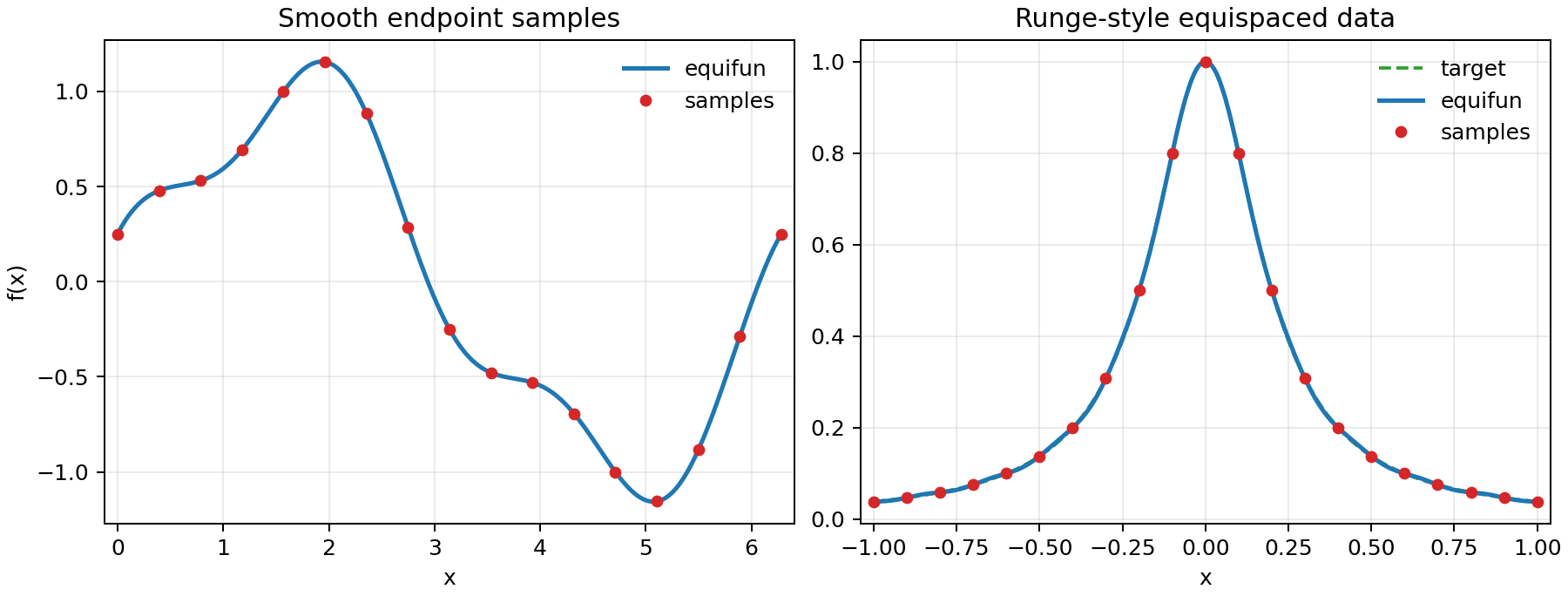
nodes = np.linspace(0.0, 2.0 * np.pi, 17)
values = np.sin(nodes) + 0.25 * np.cos(3.0 * nodes)
f = equifun(values, [0.0, 2.0 * np.pi])

xx = np.linspace(0.0, 2.0 * np.pi, 500)
plt.plot(xx, f(xx), label="equifun")
plt.plot(nodes, values, "o", label="samples")
plt.legend()
plt.savefig("docs/assets/equifun-examples.png", dpi=180)
For equispaced data, ChebPy first builds a Floater-Hormann rational interpolant through the samples and then adaptively represents it as a Chebfun. This is often more stable than high-degree polynomial interpolation on equispaced nodes, including Runge-style data:
Special Constructors
# Identity function
x = chebfun("x")

# Constant function
c = chebfun(3.14)

# Piecewise-constant function
from chebpy import pwc

f = pwc(domain=[-2, -1, 0, 1, 2], values=[-1, 0, 1, 2])
Multi-Interval Functions
ChebPy can represent functions with breakpoints as piecewise Chebyshev expansions:
f = chebfun(lambda x: np.abs(x), [-1, 0, 1])
Accuracy and Preferences
Adaptive construction samples the function on Chebyshev grids of length
2**k + 1. It converts the samples to Chebyshev coefficients and stops when
the coefficient tail can be chopped below a tolerance. The default tolerance is
roughly machine epsilon:
from chebpy import UserPreferences

prefs = UserPreferences()
prefs.eps  # default: numpy.finfo(float).eps
prefs.maxpow2  # default: 16, so the largest grid has 65537 points
Use the preferences object to change these defaults:
from chebpy import UserPreferences

prefs = UserPreferences()
prefs.eps = 1e-12
prefs.maxpow2 = 17

# Restore one setting, or all settings:
prefs.reset("eps")
prefs.reset()
Preferences are global. For temporary changes, use the object as a context manager:
from chebpy import UserPreferences, chebfun

prefs = UserPreferences()

with prefs as local_prefs:
    local_prefs.eps = 1e-12
    f = chebfun(lambda x: x**2)

# eps is restored here
eps is a construction tolerance, not a certified maximum error. It controls
the coefficient chopping test used during construction, but the final pointwise
error also depends on smoothness, conditioning, floating-point roundoff, and
whether the function is resolved on the chosen interval. ChebPy does not
currently provide a certified maximum-error bound. In practice, validate
sensitive approximations against extra sample points:
import numpy as np
from chebpy import chebfun


def g(x):
    return 0.3 + 0.02 * x + abs(x) ** 1.8


f = chebfun(g, [-1, 1])
x_test = np.linspace(-1, 1, 1001)
err_est = np.max(np.abs(g(x_test) - f(x_test)))
This is an error estimate over the selected test points, not a bound between them. Denser or problem-specific validation points may be needed when the function has narrow or rapidly varying features.
The adaptive constructor also uses an absolute zero test. On each interval it
sets the approximation to zero when all sampled values have magnitude at most
eps * max(hscale, 1), where hscale is ChebPy's horizontal scale for that
interval. Raising eps can therefore erase functions whose overall amplitude
is smaller than this threshold, even when their relative variation matters.
Lowering eps below its default, numpy.finfo(float).eps, may request a longer
polynomial and reduce truncation error for a difficult function, but it cannot
provide floating-point accuracy beyond machine precision. The requested
tolerance is then below roundoff and may simply drive construction to
maxpow2. Use independent validation to decide whether the longer
approximation is useful.
The example above is deliberately difficult at x = 0: abs(x)**1.8 is not
twice differentiable there. A single global polynomial therefore converges only
algebraically, and its largest interpolation error can occur near the cusp even
though the function is continuous. If you know the location of the nonsmooth
point, add it as a breakpoint:
f = chebfun(g, [-1, 0, 1])
Here the breakpoint moves the fractional-power singularity from the interior to the endpoints of two pieces. Those pieces are still not fully smooth, so their convergence remains algebraic, but the split usually reduces the interpolation error substantially. When a function consists of genuinely smooth branches, breakpoints let ChebPy approximate each branch separately.
If construction remains unresolved at maxpow2, ChebPy emits this warning:
The Chebtech constructor did not converge: using 65537 points
Treat this as a resolution warning. The returned object contains the largest
sampled interpolant, but ChebPy has not seen coefficient decay strong enough to
declare it resolved. For a smooth but highly oscillatory function, increasing
maxpow2 may be appropriate. For a nonsmooth function, add breakpoints at
known kinks or jumps. For supported endpoint singularities, use the specialized
sing= construction. For noisy or discontinuous data, a
polynomial interpolant may not be the right model.
Chebyshev Points
Use chebpts to get the Chebyshev interpolation points and barycentric weights:
from chebpy import chebpts

pts, wts = chebpts(16)  # 16 points on [-1, 1]
pts, wts = chebpts(16, [0, 3])  # 16 points on [0, 3]
References
- Z. Battles and L. N. Trefethen, An extension of MATLAB to continuous functions and operators, SIAM J. Sci. Comput., 25 (2004), pp. 1743–1770.
- L. N. Trefethen, Approximation Theory and Approximation Practice, SIAM, 2013 (extended edition 2019).
- J. L. Aurentz and L. N. Trefethen, Chopping a Chebyshev series, ACM Trans. Math. Softw., 43 (2017), Article 33.
- R. Pachón, R. B. Platte, and L. N. Trefethen, Piecewise-smooth chebfuns, IMA J. Numer. Anal., 30 (2010), pp. 898–916.